|
by phorneker
Introduction to TeX/LaTeX showed us what the TeX typesetting system was and how it works with a rather simple example of a TeX/LaTeX document.
In that article, I mentioned the project called Mathematical Approach to Photography that was created for a mathematical modeling class I took in my senior year in college. At that time, the way to digitize photographs was to scan them in using bulky image scanners that were connected through either a proprietary interface, or through a SCSI controller.
Most photographs at that time were taken on film, and image scanners were prohibitively expensive for the consumer.
It is that project that I will use in this article to show what TeX can do.
For this article, I shall use Texmaker for development of the document. Texworks, Texstudio and LyX are all available in the repository, but Texmaker is widely used for TeX development and provides a work environment that allows us to see a complete overview of the project.
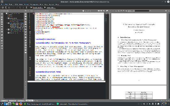
Here, we have the preamble to the document:
\documentclass[12pt,letterpaper]{article}
\usepackage[utf8]{inputenc}
\usepackage{amsmath}
\usepackage{amsfonts}
\usepackage{amssymb}
\usepackage{graphicx}
\usepackage[left=1in,right=1in,top=1in,bottom=1in]{geometry}
\author{Patrick G Horneker}
\title{A Mathematical Approach to Photography\\Revised for the 21st Century}
For this document, I chose letter paper (the standard 8½ x 11 inch size) as the paper for printing this document, and this will be typeset as an article with a 12 point font for normal text and UFT8 encoding (as opposed to the much older ASCII coding) for documents.
The standard AMS packages are used as is the graphicx and geometry packages. The graphicx package allows for PNG and JPEG images to be embedded in TeX documents.
The geometry package allows for setting of margins on a page. Here, one inch margins are set for the document as opposed to the default two inch margins.
Why is the default margin set at two inches? The answer to this can be found when documents are bound with a three ring binder. When holes are punched in standard 8½ x 11 inch paper, the left margin must be increased by one inch to accommodate the holes. The right margin allows for the reader to annotate text.
Hence the available space for typesetting is actually 6½ x 9 inches.
Remember taking college level exams in blue books?
Many colleges and universities provide blue books for writing answers to exam questions. These books are sixteen pages (four sheets of special paper folded to create the 16 pages) bound by a blue cover with the name of the institution and spaces to write the name of the course, instructor, your name and of course, the grade for the exam.
Each page was 61/2 inches width x 9 inches in length. Coincidence?
|
The following statement sets the document to one inch margins the same as any word processing package (such as LibreOffice) does.
\usepackage[left=1in,right=1in,top=1in,bottom=1in]{geometry}
If we really wanted to set the margins to what LibreOffice uses for its defaults, we could set the \usepackage statement to:
\usepackage[left=.75in,right=.75in,top=.75in,bottom=.75in]{geometry}
Now, let us look at the title statement.
\title{A Mathematical Approach to Photography\\Revised for the 21st Century}
There are two forward slashes in the middle of the title. This is done to (properly) split the title into two lines. If the slashes were not there, not only the word Revised here would have appeared on the first line, the title would have been too long to fit on just one line (and an error message would have resulted and/or the title would have been chopped at the ends).
The \maketitle statement renders the title at the beginning of the document. Had I declared the document to be of type book rather than of type article, the title would have been rendered as a separate page rather than being rendered at the top of the first page of this document.

With the book class, page numbers appear at the upper left hand corner of the page on even numbered pages and at the upper right hand corner of the page on odd numbered pages.
In addition, the geometry package overrides the defaults for typesetting in the book class, not just the article class. (Let us now revert back to the article class in the document to continue.)
Note that the numbering of sections, subsections, parts and chapters in the book class start with zero as opposed to numbering starting with one in the article class.
Next, let us look the sectioning. The statements:
\section{Introduction}
and
\subsection{What Has Mathematics Got To Do With Photography?}
have been numbered starting with one. But, does the numbering really matter here? Let us modify the \section statement so it reads
\section*{Introduction}
...and save the document. Now, build the document.

Two things happened here. The numbering for Introduction was turned off as expected. However, the numbering was reset so it starts at zero rather than one, and all other sections were renumbered accordingly.
Hence, the presence of numbering here really did make a difference. Let us reset the numbering in the Introduction header. Now everything is as expected. Let us go the next section called How Big is that Photograph?
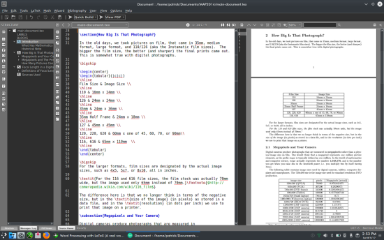
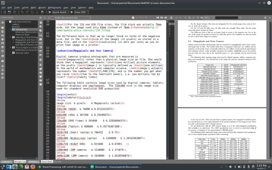
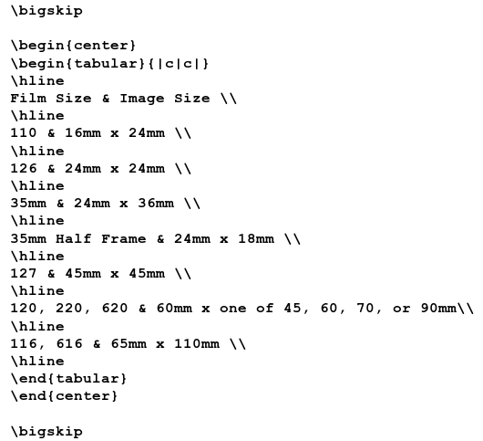
The \bigskip statement is used to provide (plenty of) space between text and the tables.
Here, we have a block of LaTeX code that defines a table embedded into the document. In this block, we define two TeX/LaTeX environments.
The first TeX environment starts with a \begin{center} and ends with \end{center}. Everything contained within this environment is horizontally centered on the page. This particular environment is defined to center a table on the page. You can use this statement to center blocks of text, mathematical formulas, graphics or anything else contained within on that part of the document.
The second TeX environment starts with \begin{tabular}{|c|c|} and ends with \end{tabular}. The tabular parameter in the begin and end statements here tells TeX that the following block defines a table rather than ordinary text. Also, the tabular statement contains an additional parameter contained in its own set of braces that defines the table structure.
Tables are graphically defined with the borders between columns indicated by a |. Text contained within the columns is justified by a parameter, which could be l, r, or c, where:
Lower case l means left justified, lower case r leans right justified, and lower case c means centered. In this case, there are three columns, all columns contain centered text.
The actual table is defined as follows:
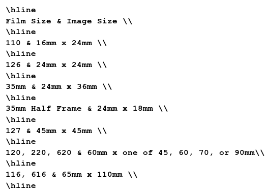
The \hline statements provide the top and bottom lines that define the borders of each cell in the table. The | in the \begin{tabular}{|c|c|} statement provide the left and right borders of each cell.
Each line in the tabular environment defines a row in the table, with each of the rows separated by two forward slashes (\\). Columns in each row are separated by an ampersand (&).
The center environment is optional. Without the center environment, the table would be left justified on the page (at the beginning of where normal paragraphs start).
In this case, the center environment is necessary to make the table easier to spot and read.
Moving further into the document, we notice a footnote. The \footnote{$http://camerapedia.wikia.com/wiki/116_film$} statement first tells TeX there that there is a URL contained in the footnote (indicated the the leading and trailing $, and where in the document to place the footnote markers (in the text as well as on the footnote itself).
Footnotes are generally typeset with the footnote at the bottom of the page and its corresponding marker on the same page.
In computer science, a kilobyte is defined as 1,024 bytes instead of 1,000 as most of us would think. The number 1,024 is two to the 10th power (210=1024), or what you get when you multiply two by itself ten times.
Likewise, two to the twentieth power 220=1,048,576defines a megabyte, and hence, the prefix mega- in computer science refers to the number 1,048,576 instead of 1,000,000 as one would think.
...and therefore, a megapixel is defined as 1,048,576 pixels (or picture elements). This is the figure I used to calculate the megapixel values in this table.
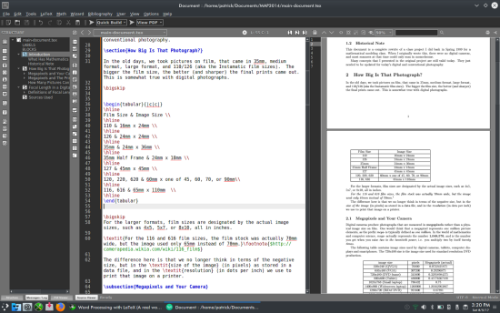
|
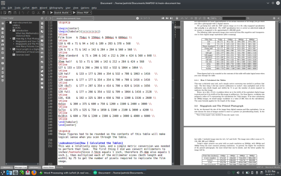
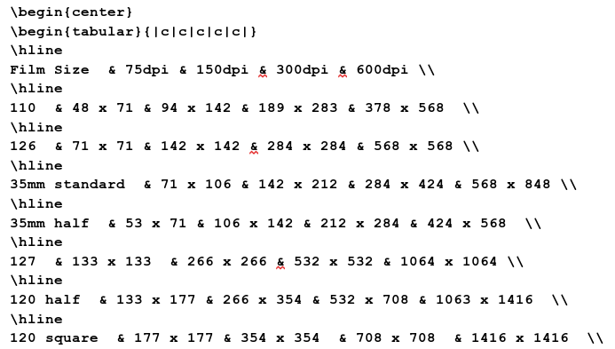
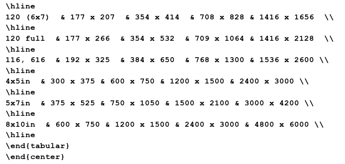
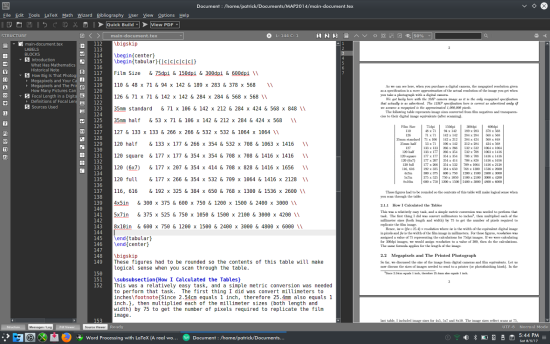
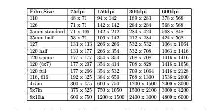
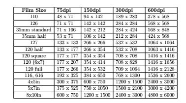
Let us look at another table and its contents. The lines look like a mess, but there are five columns per row on this table. This is a table of scanned image sizes in terms of width and height in pixels. The x are not delimiters for the rows, but are necessary to show the width and height dimensions as one cell entry. Cell entries are delimited by an ampersand (&), and rows are delimited by two forward slashes (\\).
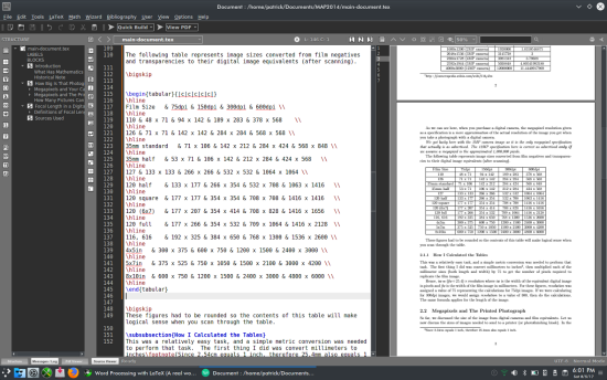
In the document preview panel, the table is neatly formatted and entries are easy to spot. What happens when we remove the \hline statements?
You can still read the table, but now we have only vertical lines to separate the columns. It does not look as good, but the table is still readable.
Now, take out the vertical lines so the \begin{tabular} statement reads as:
\begin{tabular}{ccccc}
...then rebuild the document and this is what happens:
You can still read the table, but it stands out better with the lines in. By adding and deleting a combination of \hline statements within the table and/or modifying the second parameter in the \begin{tabular} statement, we can create some useful effects to the tables.
Suppose we change \begin{center} to \begin{flushright}. If we do this, we must also change \end{center} to \end{flushright} or we will get an error message (not to mention a messed up document in appearance). We get something like this:

Let us now change the \begin{flushright} to \begin{flushleft} (and do likewise to the corresponding \end statement), we get this:

So what happens when we remove the \begin{flushleft} statement? One would think the table would be positioned the same. Not quite!
Having the \begin{flushleft} statement instead of simply removing the statement does make a difference.
The \begin{flushleft} statement places the table at the left margin on the page rather than the table being aligned to the beginning of a normal paragraph as not having the \begin{flushleft} statement would do.
Let us go back to the \begin{tabular}{|c|c|c|c|c|} statement. The second parameter defines the format for which columns in the table are displayed. Without any parameters, TeX will generate an error message. Hence, there must be at least one column alignment value present in the second parameter for a table to be typeset.
Valid column alignment values are c, l, and r for centered, left and right alignment respectively. The | is optional, and when present, typesets a vertical line in the table.
For the table to be typeset successfully, the second parameter in the \begin{tabular} statement must have one column alignment value for every column represented in the table itself. As ampersands (&) delimit columns, each row in the table must contain one fewer ampersands than the number of columns in the row data.
In this example, there are five columns for each row. For the table to typeset successfully, there must be four ampersands in each row.
Let us look further at the \begin{tabular}{|c|c|c|c|c|} statement. The number of | characters depends on how many vertical lines you wish to typeset. In this example, the \begin{tabular}{|c|c|c|c|c|} statement typesets vertical lines between columns. If we remove all but the two outermost | characters, we will have a single border around the entire table.
We can change each of the values in the second parameter. Suppose we decide to left align each of the cells in this table. The \begin{tabular} statement will read as follows:
\begin{tabular}{|l|l|l|l|l|}
...and will result in this:
On the first row of the table, it is a good idea to highlight the data in the first row of this table as this data row is a row of column titles represented in the table.
\textbf{Film Size} & \textbf{75dpi} & \textbf{150dpi} & \textbf{300dpi} & \textbf{600dpi} \\
Each column must be typeset by enclosing the column data inside a \textbf{}. Let us rebuild this document and see the changes to the table.
The titles in each of the columns are now in boldface as expected. (You may not be able to see this in this graphic, but the result is there.) Let us change the first column only so the labels are centered. The \begin{tabular} statement should read as follows:
Screenshot_20170806_202120.png
\begin{tabular}{|c|l|l|l|l|}
Now the table should look like this (after rebuilding):
Let us look at the subsection below the table we just modified:
Below is the LaTeX code to create this part of the document.
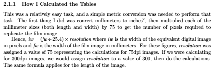
\subsubsection{How I Calculated the Tables}>br?
This was a relatively easy task, and a simple metric conversion was needed to perform that task. The first thing I did was convert millimeters to inches\footnote{Since 2.54cm equals 1 inch, therefore 25.4mm also equals 1 inch.}, then multiplied each of the millimeter sizes (both length and width) by 75 to get the number of pixels required to replicate the film image.
Hence, $\textit{iw} = (\textit{fw} \div 25.4) \times \textit{resolution}$ where \textit{iw} is the width of the equivalent digital image in pixels and \textit{fw} is the width of the film image in millimeters. For these figures, \textit{resolution} was assigned a value of 75 representing the calculations for 75dpi images. If we were calculating for 300dpi images, we would assign \textit{resolution} to a value of 300, then do the calculations. The same formula applies for the length of the image.
|
The \paragraph statement from the last article is not really needed to typeset this document. This LaTeX fragment contains a number of formatting commands, and has an example of how a mathematical formula is typeset.
Mathematical formulas are one of the greatest strengths of the TeX/LaTeX typesetting system. The $ tells TeX that what follows, until another $ is encountered, is a mathematical formula.
In this example, $\textit{iw} = (\textit{fw} \div 25.4) \times \textit{resolution}$ is typeset as a formula, namely
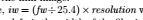
In a typical mathematical publication (of those that I have come across), variables are usually typeset in italics, hence the \textit{} statements.
|
There is another \footnote{} statement in this section as well. This footnote refers to a simple conversion from inches to millimeters, specifically if there are 2.54cm to an inch, it then follows that there are 25.4 millimeters to that same inch.
|
Another example of a formula appears in the next section of this document. This one involves the Pythagorean Theorem.
...and here is the TeX/LaTeX code that generated this:
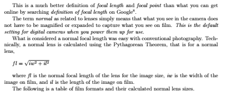
This is a much better definition of \textit{focal length} and \textit{focal point} than what you can get online by searching \textit{definition of focal length} on Google\footnote{This is more proof that you cannot always rely on the Internet for everything. The Wikipedia definition is even worse.}.
The term \textit{normal} as related to lenses simply means that what you see in the camera does not have to be magnified or expanded to capture what you see on film. \textit{This is the default setting for digital cameras when you power them up for use}.
What is considered a normal focal length was easy with conventional photography. Technically, a normal lens is calculated using the Pythagorean Theorem, that is for a normal lens,
\bigskip
$fl= \sqrt{iw^2+il^2}$
\bigskip
where \textit{fl} is the normal focal length of the lens for the image size, \textit{iw} is the width of the image on film, and \textit{il} is the length of the image on film.
The following is a table of film formats and their calculated normal lens sizes.
|
The formula being typeset here is:
$fl= \sqrt{iw^2+il^2}$
The \sqrt{} command typesets the formula enclosed in {}, then draws a square root symbol encompassing the entire formula in the document. (Try that with LibreOffice.)
Just above this formula is an example of what Tex/LaTeX does with the text between \begin{quote} and \end{quote} statements.
\begin{quote}
When a simple lens is held so that an image of the sun, or any very distant object, is focused sharply on a cardboard, the image is at the \textit{principal focus} and the distance from the cardboard to the lens is the \textit{focal length} of that lens.
\end{quote}
|
...yields this in the document:
What happened? The quote environment indented the text by one half-inch in both the left and right margins.
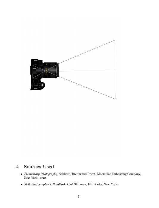
In the last part of this sample document, there are two more features of TeX/LaTeX that are available in TexLive. The graphics package allows for graphics to be embedded in theTeX/LaTeX document.
\includegraphics[scale=.5]{angle-of-view.png}
Texmaker has a command in the LaTeX menu that allows you to use this command. Select a file from the dialog box that comes up. The embedded graphic must be in the same directory as the LaTeX files, and must be in a supported format (EPS, JPG and PNG are acceptable).
Finally, the following segment of LaTeX code produces the bibliography (or works cited) section commonly found in many documents that are typeset using this system.
\section{Sources Used}
\begin{itemize}
\item \textit{Elementary Photography}, Neblette, Brehm and Priest, Macmillan Publishing Company, New York, 1940.
\item \textit{SLR Photographer's Handbook}, Carl Shipman, HP Books, New York.
\end{itemize}
The itemize environment produces a bulleted list. Items to be bulleted start with the \item command and end with the next \item command, or with the \end{itemize} statement.
As we can see, there is a lot more work to be done on this project. What I have presented to you is some of what TeX and LaTeX can do for your typesetting projects.
The document, so far, produces a PDF that is seven pages in length. This is with setting the margins to one inch and using a 12 point Computer Modern font.
Below is the actual LaTeX code that produces the seven page document.
\documentclass[12pt,letterpaper]{article}
\usepackage[utf8]{inputenc}
\usepackage{amsmath}
\usepackage{amsfonts}
\usepackage{amssymb}
\usepackage{graphicx}
\usepackage[left=1in,right=1in,top=1in,bottom=1in]{geometry}
\author{Patrick G Horneker}
\title{A Mathematical Approach to Photography\\Revised for the 21st Century}
\begin{document}
\maketitle
\section{Introduction}
\subsection{What Has Mathematics Got To Do With Photography?}
Some of you are probably asking this very question. The answer to that is quite simple: \textit{everything}. One could argue that photography is an art. That is true. However, it is an art that involves some significant technical knowledge of the equipment used to produce this art. Without that knowledge, could you really know what you are doing to get that great photograph?
The intent of \textit{Mathematical Approach to Photography} is to explain the mathematics involved in every aspect of making a photograph, from the size of the film (or digital) image, to calculating the shutter speed and aperture settings, to printing the final product (be it a digital print on an inkjet printer, or exposing and developing a photograph in a darkroom).
\subsection{Historical Note}
This document is a complete rewrite of a class project I did back in Spring 1989 for a mathematical modeling class. When I originally wrote this, there were no digital cameras, and most scanners at that time could only scan in monochrome.
Many concepts that I presented in the original project are still valid today. They just needed to be updated for today's digital and conventional photography.
\section{How Big Is That Photograph?}
In the old days, we took pictures on film, that came in 35mm, medium format, large format, and 110/126 (aka the Instamatic film sizes). The bigger the film size, the better (and sharper) the final prints came out. This is somewhat true with digital photographs.
For the larger formats, film sizes are designated by the actual image sizes, such as 4x5, 5x7, or 8x10, all in inches.
\textit{For the 116 and 616 film sizes, the film stock was actually 70mm wide, but the image used only 65mm instead of 70mm.}\footnote{$http://camerapedia.wikia.com/wiki/116_film$}
The difference here is that we no longer think in terms of the negative size, but in the \textit{size of the image} (in pixels) as stored in a data file, and in the \textit{resolution} (in dots per inch) we use to print that image on a printer.
\subsection{Megapixels and Your Camera}
,br>
Digital cameras produce photographs that are measured in \textbf{megapixels} rather than a physical image size on film. One would think that a megapixel represents \textit{one million} picture elements, as the prefix \textit{mega-} is typically defined as \textit{one million}. In the world of mathematics and computer science, \textit{mega-} actually represents the number \textbf{1,048,576}, and is the number you get when you raise \textit{two to the twentieth power}, i.e. you multiply two by itself \textit{twenty times}.
The following table contains image sizes used by digital cameras, tablets, computer displays and smartphones. The 720x480 size is the image size used for standard resolution DVD production.
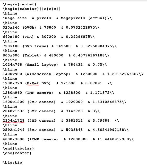
As we can see here, when you purchase a digital camera, the megapixel resolution given as a specification is a \textit{mere approximation} of the actual resolution of the image you get when you take a photograph with a digital camera.
\textit{We got lucky here with the 3MP camera image as it is the only megapixel specification that actually is as advertised. The 12MP specification here is correct as advertised \textbf{only if} we assume a megapixel is the approximated 1,000,000 pixels.}
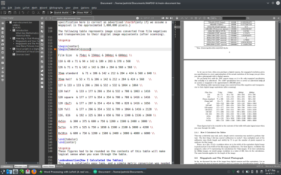
The following table represents image sizes converted from film negatives and transparencies to their digital image equivalents (after scanning).
These figures had to be rounded so the contents of this table will make logical sense when you scan through the table.
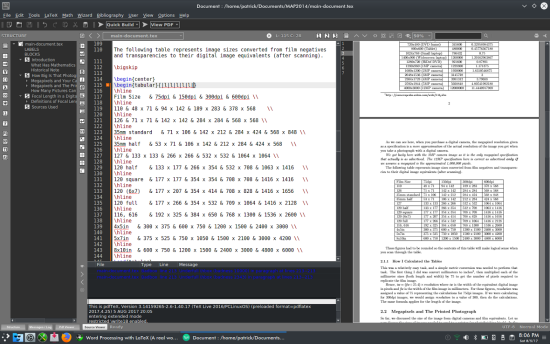
\subsubsection{How I Calculated the Tables}
This was a relatively easy task, and a simple metric conversion was needed to perform that task. The first thing I did was convert millimeters to inches\footnote{Since 2.54cm equals 1 inch, therefore 25.4mm also equals 1 inch.}, then multiplied each of the millimeter sizes (both length and width) by 75 to get the number of pixels required to replicate the film image.
,br>
Hence, $\textit{iw} = (\textit{fw} \div 25.4) \times \textit{resolution}$ where \textit{iw} is the width of the equivalent digital image in pixels and \textit{fw} is the width of the film image in millimeters. For these figures, \textit{resolution} was assigned a value of 75 representing the calculations for 75dpi images. If we were calculating for 300dpi images, we would assign \textit{resolution} to a value of 300, then do the calculations. The same formula applies for the length of the image.
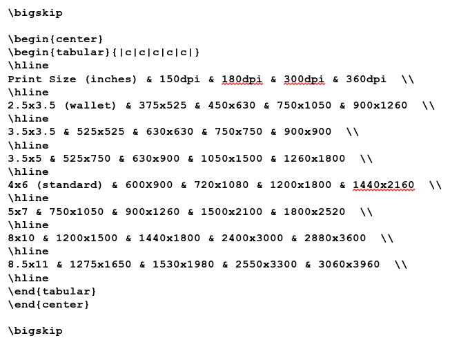
\subsection{Megapixels and The Printed Photograph}
So far, we discussed the size of the image from digital cameras and film equivalents. Let us now discuss the sizes of images needed to send to a printer (or photofinishing kiosk). In the last table, I included image sizes for 4x5, 5x7 and 8x10. The image sizes reflect scans at 75, 150, 300, 600 and 1200dpi.
Today's inkjet printers can print with as much resolution as 2880dpi, with 300dpi and 360dpi being the most common printing resolutions. In general, the higher the resolution of the printed photograph, the more detail that can be shown, and the better quality the image will be.
\subsubsection{This is all Theoretical}
Of course, these figures calculated based on the full usage of available space in each size of the photograph. These figures do not take into account differences in hardware design (or glitches for that matter) or software handling of digital images.
\subsection{How Many Pictures Can I Take With a Memory Card?}
When digital cameras first came out, this was \textbf{the most frequently asked question} I was asked by the general public.
Unlike conventional film, there is \textbf{no definitive answer} to this question. With a roll of 35mm film, you got 12, 24 or 36 exposures on a roll\footnote{Even here, there are some exceptions. If you had a Bolsey B3 camera, you could get an additional three exposures on a roll because of the short path between the 35mm cartridge and the spool on the other side of the camera.} The size of the negative (or transparency) image was always the same, namely 24mmx36mm\footnote{There were very few 35mm cameras ever made that took half-frame exposures. For those cameras, the image size was 18mmx24mm.}.
Digital cameras...
\begin{itemize}
\item can take more than one size of digital picture.
\item will tell you how many pictures you can store on the memory card you have inserted \textit{based on the current resolution} you set, usually the maximum available for the camera.
\item will let you delete unwanted pictures without removing the memory card.
\end{itemize}
Even with all images the same physical size, no two pictures on a memory card take up the \textit{exact amount of space}. This depends on the method your camera uses to compress digital images to JPEG format\footnote{I have yet to see a digital camera that can compress to PNG or TIFF.}. In addition, your camera may add additional information to the image file\footnote{In the form of EXIF tags, a topic for another section on this document.}.
\section{Focal Length in a Digital Camera}
\subsection{Definitions of Focal Length and Focal Point}
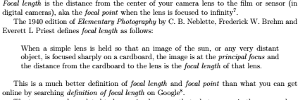
\textit{Focal length} is the distance from the center of your camera lens to the film or sensor (in digital cameras), aka the \textit{focal point} when the lens is focused to infinity\footnote{This concept is best explained at http://www.nikonusa.com/en/Learn-And-Explore/Article/g3cu6o2o/understanding-focal-length.html. The dictionaries, both book form and online do not provide a concise definition of \textit{focal point} as it relates to photography.}.
The 1940 edition of \textit{Elementary Photography} by C. B. Neblette, Frederick W. Brehm and Everett L Priest defines \textit{focal length} as follows:
\begin{quote}
When a simple lens is held so that an image of the sun, or any very distant object, is focused sharply on a cardboard, the image is at the \textit{principal focus} and the distance from the cardboard to the lens is the \textit{focal length} of that lens.
\end{quote}
This is a much better definition of \textit{focal length} and \textit{focal point} than what you can get online by searching \textit{definition of focal length} on Google\footnote{This is more proof that you cannot always rely on the Internet for everything. The Wikipedia definition is even worse.}.
The term \textit{normal} as related to lenses simply means that what you see in the camera does not have to be magnified or expanded to capture what you see on film. \textit{This is the default setting for digital cameras when you power them up for use}.
What is considered a normal focal length was easy with conventional photography. Technically, a normal lens is calculated using the Pythagorean Theorem, that is for a normal lens,
\bigskip
$fl= \sqrt{iw^2+il^2}$
\bigskip
where \textit{fl} is the normal focal length of the lens for the image size, \textit{iw} is the width of the image on film, and \textit{il} is the length of the image on film.
The following is a table of film formats and their calculated normal lens sizes.
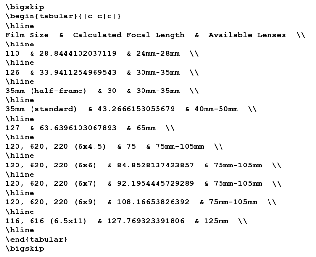
Some medium format cameras utilize interchangeable film backs, hence the available lenses are the same for the 6x4.5 to 6x9 film sizes. Digital film backs for such cameras are available so the same camera can be used to produce both film and digital images (not to mention to protect the investment in the cost of the camera).
The ranges shown in the table represent the available lens focal lengths for film cameras that the manufacturer considers to be \textit{normal}.
What is considered to be a normal lens for digital cameras \textit{has not been officially defined}, though it has been reported to be between 6mm and 10mm for most inexpensive digital cameras. Digital SLRs typically have normal lenses of 35mm (the focal length and not the film size).
But then, how can we define a focal length for a normal lens if the image size of a digital camera is arbitrary\footnote{As discussed in the last section, digital image sizes vary by the camera.}.
Your camera documentation (user manual) should have that information available (unless it is a bargain basement model without an LCD screen, in which case the lens is already fixed at what the manufacturer considers to be normal).
\subsubsection{Digital Cameras With Adjustable Focal Lengths}
Many digital cameras have a zoom feature\footnote{If you have a digital SLR camera, this is inherent with the purchase of additional lenses for that camera.}. There are two types of zooming on digital cameras\footnote{For digital SLRs, there is only the optical zoom, and that depends on the lens attached to the camera.}.
Digital zoom only simulates adjustment of the focal length by reducing the size of the digital image. Think of a rectangle expanding outward from and zooming in towards the center of the image. The image that appears in the rectangle is what the digital camera captures with digital zoom when you take that picture.
Cameras with optical zoom have an actual zoom lens that is either built in to the camera, or is a digital camera with interchangeable lenses. Zooming with one of these cameras is done without degrading the quality of the image.
\includegraphics[scale=.5]{angle-of-view.png}
\section{Sources Used}
\begin{itemize}
\item \textit{Elementary Photography}, Neblette, Brehm and Priest, Macmillan Publishing Company, New York, 1940.
\item \textit{SLR Photographer's Handbook}, Carl Shipman, HP Books, New York.
\end{itemize}
\end{document}
...oh, and let us not forget the graphic.
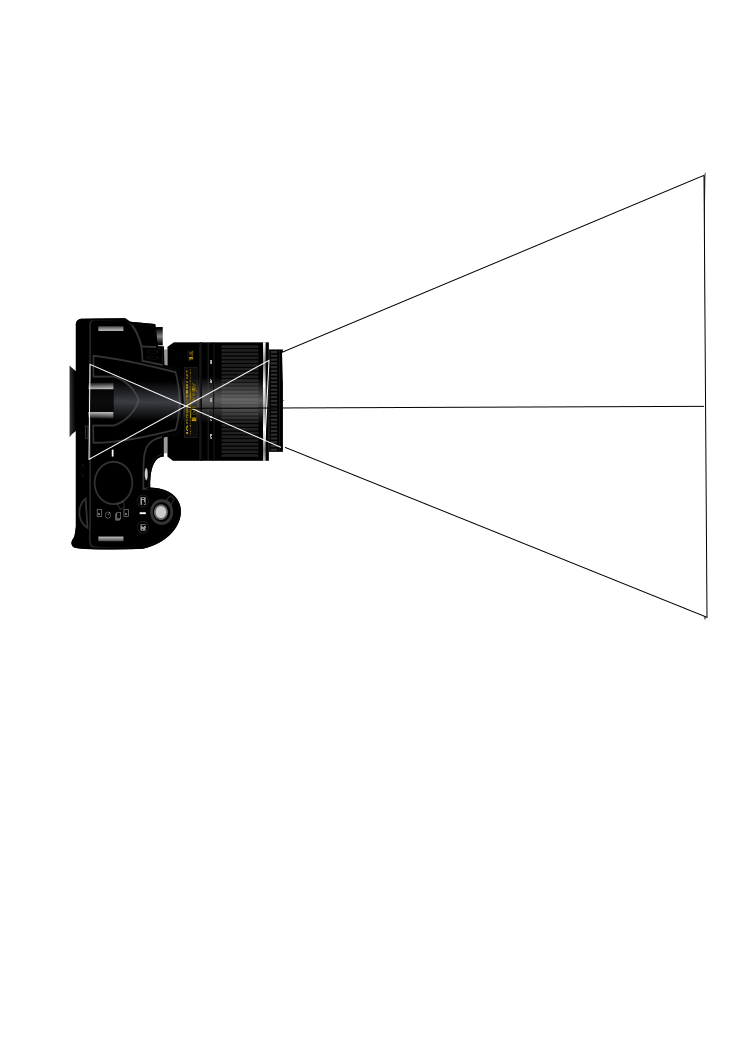
|